Chapter 1 Probability
1.1 Load packages, load data, set theme
Let’s load the packages that we need for this chapter.
library("knitr")        # for rendering the RMarkdown file
library("kableExtra")   # for nicely formatted tables
library("arrangements") # fast generators and iterators for creating combinations
library("DiagrammeR")   # for drawing diagrams
library("tidyverse")    # for data wrangling
## Warning: package 'ggplot2' was built under R version 4.3.1## Warning: package 'dplyr' was built under R version 4.3.1Set the plotting theme.
1.2 Learning goals
I like to think of statistics as “applied epistemology”, the art of making precise statements about what we can and can’t “know” from limited and noisy observations. When we’re trying to do science under these conditions, we’re usually expressing our (lack of) knowledge as uncertainty. We’re often not sure whether there’s really an effect in our experiments, or how big it might be. We can measure a number, but we know that if we did the experiment again, we would get a slightly different number. Probability theory gives us a language for talking about these concepts in a less hand-wavy way; it helps us quantify uncertainty. Probabilities are the conceptual foundation of everything we’re going to do in this course, and we’re going to start out by learning to look at the phenomena from PSYCH 610 from a different perspective.
1.3 Counting
Imagine that there are three balls in an urn. The balls are labeled 1, 2, and 3. Let’s consider a few possible situations.
balls = 1:3 # number of balls in urn
ndraws = 2 # number of draws

# order matters, without replacement
permutations(balls, ndraws)
[,1] [,2]
[1,] 1 2
[2,] 1 3
[3,] 2 1
[4,] 2 3
[5,] 3 1
[6,] 3 2 [,1] [,2]
[1,] 1 1
[2,] 1 2
[3,] 1 3
[4,] 2 1
[5,] 2 2
[6,] 2 3
[7,] 3 1
[8,] 3 2
[9,] 3 3 [,1] [,2]
[1,] 1 1
[2,] 1 2
[3,] 1 3
[4,] 2 2
[5,] 2 3
[6,] 3 3 [,1] [,2]
[1,] 1 2
[2,] 1 3
[3,] 2 3I’ve generated the figures below using the DiagrammeR package. It’s a powerful package for drawing diagrams in R. See information on how to use the DiagrammeR package here.
Figure 1.1: Drawing two marbles out of an urn with replacement.
Figure 1.2: Drawing two marbles out of an urn without replacement.
1.4 Sampling
We can also draw samples from the urn:
[1] 2 1 2 2 1 2 2 3 1 1Use the prob = argument to change the probability with which each number should be drawn.
[1] 1 1 1 1 1 3 1 1 1 1Make sure to set the seed in order to make your code reproducible. The code chunk below may give a different outcome each time is run.
[1] 5 2 1 3 4The chunk below will produce the same outcome every time it’s run.
[1] 1 4 3 5 21.4.1 Drawing rows from a data frame
We can do this with data frames too, imagining our data frame is the urn and the rows are balls.
set.seed(1)
n = 10
df.data = tibble(trial = 1:n,
                 stimulus = sample(c("flower", "pet"), size = n, replace = T),
                 rating = sample(1:10, size = n, replace = T))
Sample a given number of rows.
# A tibble: 6 × 3
  trial stimulus rating
  <int> <chr>     <int>
1     9 pet           9
2     4 flower        5
3     7 flower       10
4     1 flower        3
5     2 pet           1
6 7 flower 10# A tibble: 5 × 3
trial stimulus rating
<int> <chr> <int>
1 9 pet 9
2 4 flower 5
3 7 flower 10
4 1 flower 3
5 2 pet 11.5 More complex counting / matching
Imagine a secretary types four letters to four people and addresses the four envelopes. If they insert the letters at random, each in a different envelope, what is the probability that exactly three letters will go into the right envelope?
df.letters = permutations(x = 1:4, k = 4) %>%
  as_tibble(.name_repair = ~ str_c("person_", 1:4)) %>%
  mutate(n_correct = (person_1 == 1) +
           (person_2 == 2) +
           (person_3 == 3) +
           (person_4 == 4))

df.letters %>%
  summarize(prob_3_correct = sum(n_correct == 3) / n())
# A tibble: 1 × 1
prob_3_correct
<dbl>
1 0ggplot(data = df.letters,
mapping = aes(x = n_correct)) +
geom_bar(aes(y = stat(count)/sum(count)),
color = "black",
fill = "lightblue") +
scale_y_continuous(labels = scales::percent,
expand = c(0, 0)) +
labs(x = "number correct",
y = "probability")Warning: `stat(count)` was deprecated in ggplot2 3.4.0.
ℹ Please use `after_stat(count)` instead.
This warning is displayed once every 8 hours.
Call `lifecycle::last_lifecycle_warnings()` to see where this warning was generated.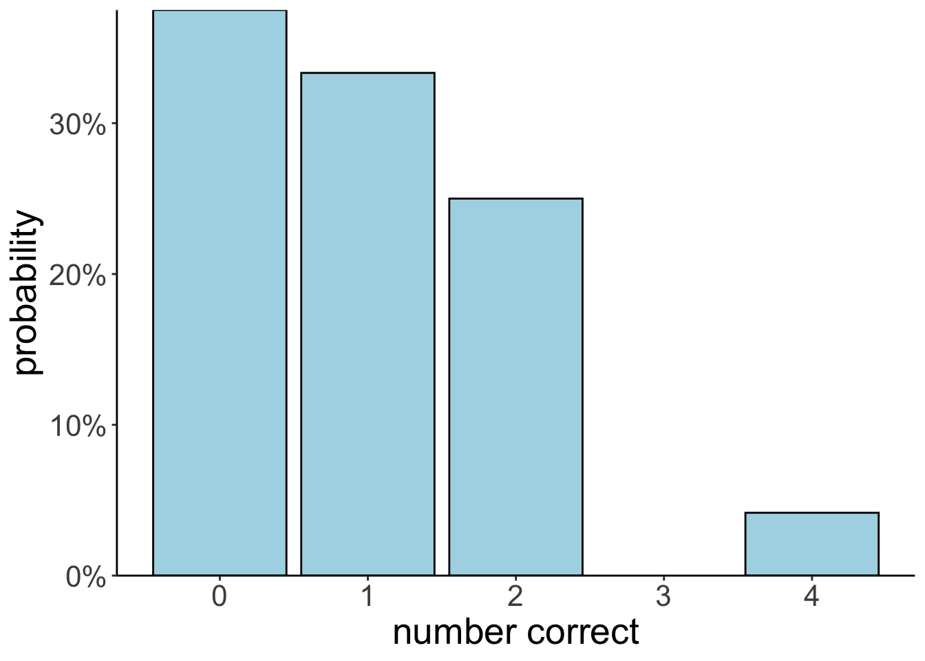
1.6 Conditional probability
who = c("ms_scarlet", "col_mustard", "mrs_white",
        "mr_green", "mrs_peacock", "prof_plum")
what = c("candlestick", "knife", "lead_pipe",
         "revolver", "rope", "wrench")
where = c("study", "kitchen", "conservatory",
          "lounge", "billiard_room", "hall",
          "dining_room", "ballroom", "library")

df.clue = expand_grid(who = who,
                      what = what,
                      where = where)

df.suspects = df.clue %>%
  distinct(who) %>%
  mutate(gender = ifelse(test = who %in% c("ms_scarlet", "mrs_white", "mrs_peacock"),
                         yes = "female",
no = "male"))| who | gender |
|---|---|
| col_mustard | male |
| mr_green | male |
| prof_plum | male |
| ms_scarlet | female |
| mrs_white | female |
| mrs_peacock | female |
# conditional probability (via rules of probability)
df.suspects %>%
  summarize(p_prof_plum_given_male =
              sum(gender == "male" & who == "prof_plum") /
              sum(gender == "male"))
# A tibble: 1 × 1
p_prof_plum_given_male
<dbl>
1 0.333# conditional probability (via rejection)
df.suspects %>%
filter(gender == "male") %>%
summarize(p_prof_plum_given_male =
sum(who == "prof_plum") /
n())# A tibble: 1 × 1
p_prof_plum_given_male
<dbl>
1 0.3331.7 Law of total probability
# Make a deck of cards
df.cards = tibble(suit = rep(c("Clubs", "Spades", "Hearts", "Diamonds"), each = 8),
                  value = rep(c("7", "8", "9", "10", "Jack", "Queen", "King", "Ace"), 4))
# conditional probability: p(Hearts | Queen) (via rules of probability)
df.cards %>%
summarize(p_hearts_given_queen =
sum(suit == "Hearts" & value == "Queen") /
sum(value == "Queen"))# A tibble: 1 × 1
p_hearts_given_queen
<dbl>
1 0.25# conditional probability: p(Hearts | Queen) (via rejection)
df.cards %>%
filter(value == "Queen") %>%
summarize(p_hearts_given_queen = sum(suit == "Hearts")/n())# A tibble: 1 × 1
p_hearts_given_queen
<dbl>
1 0.251.9 Session info
Information about this R session including which version of R was used, and what packages were loaded.
R version 4.3.0 (2023-04-21)
Platform: aarch64-apple-darwin20 (64-bit)
Running under: macOS 14.1.1

Matrix products: default
BLAS:   /Library/Frameworks/R.framework/Versions/4.3-arm64/Resources/lib/libRblas.0.dylib
LAPACK: /Library/Frameworks/R.framework/Versions/4.3-arm64/Resources/lib/libRlapack.dylib;  LAPACK version 3.11.0

locale:
[1] en_US.UTF-8/en_US.UTF-8/en_US.UTF-8/C/en_US.UTF-8/en_US.UTF-8

time zone: America/Chicago
tzcode source: internal

attached base packages:
[1] stats     graphics  grDevices utils     datasets  methods   base

other attached packages:
 [1] lubridate_1.9.2    forcats_1.0.0      stringr_1.5.0      dplyr_1.1.4
 [5] purrr_1.0.2        readr_2.1.4        tidyr_1.3.0        tibble_3.2.1
 [9] ggplot2_3.4.4      tidyverse_2.0.0    DiagrammeR_1.0.10  arrangements_1.1.9
[13] kableExtra_1.3.4   knitr_1.42

loaded via a namespace (and not attached):
 [1] gmp_0.7-3          sass_0.4.6         utf8_1.2.3         generics_0.1.3
 [5] xml2_1.3.4         stringi_1.7.12     hms_1.1.3          digest_0.6.31
 [9] magrittr_2.0.3     timechange_0.2.0   evaluate_0.21      grid_4.3.0
[13] RColorBrewer_1.1-3 bookdown_0.34      fastmap_1.1.1      jsonlite_1.8.4
[17] httr_1.4.6         rvest_1.0.3        fansi_1.0.4        viridisLite_0.4.2
[21] scales_1.3.0       jquerylib_0.1.4    cli_3.6.1          crayon_1.5.2
[25] rlang_1.1.1        visNetwork_2.1.2   ellipsis_0.3.2     munsell_0.5.0
[29] withr_2.5.0        cachem_1.0.8       yaml_2.3.7         tools_4.3.0
[33] tzdb_0.4.0         colorspace_2.1-0   webshot_0.5.4      vctrs_0.6.5
[37] R6_2.5.1           lifecycle_1.0.3    htmlwidgets_1.6.2  pkgconfig_2.0.3
[41] bslib_0.4.2        pillar_1.9.0       gtable_0.3.3       glue_1.6.2
[45] systemfonts_1.0.4  highr_0.10         xfun_0.39          tidyselect_1.2.0
[49] rstudioapi_0.14    farver_2.1.1       htmltools_0.5.5    labeling_0.4.2
[53] rmarkdown_2.21     svglite_2.1.1      compiler_4.3.0